Web scraping with Python from A to Z – Part C

Part C — Storing your data and visualization

In our previous posts we gave an introduction to web scraping and how to avoid being blocked, as well as using API calls in order to enrich one’s data. In this post we will go through how to set up a database in order to store the data and how to access this data for visualization. Visualizations are a powerful tool one can use to extract insights from the data.

Previous posts:

• Part A — Handling Beautifulsoup and avoiding blocks
• Part B -Using API calls to enrich your data

Store data — MySQL DB

When setting up the database for a web scraping project (or others in general) the following should be taken into account:

• Tables creation
• New data insertion
• Data update (every hour/day…)

Tables creation

This stage of the pipeline should be done with caution and one should validate that the chosen structure (in terms of columns types, lengths, keys etc.) is suitable for the data and can handle extreme cases (missing data, non-English characters etc.). Avoid relying on an ID that is used by the website as the primary/unique key unless you have a really good reason (in our case doi_link of an article is a unique string that is acceptable everywhere, so we use it as a unique identifier of an article).

An example of tables creation using mysql.connector package:

The SQL command:

The function for building the database:

Note — in lines 12, 17, 23 and 25 we use the logger object. This is for logging to an external logs file and it’s super important. Creating a Logger class is recommended, you can see more here.

Data Insertion

Insertion of new data differs a bit from updating existing data. When new data is inserted to DB, one should make sure there are not duplicates. Also, in case of an error, one should catch it, log it and save the portion of data that caused that error for future inspection.

As seen below, we used again the cursor of mysql.connector in order to execute the SQL insert command.

Data Update

Dynamic data requires frequent updates. One should define the time deltas (differences) between two updates which depends on the data type and source. In our project, we had to take into account that the number of citations for all articles would have to be updated periodically. The following piece of code illustrates the update process:

Visualizations

In order to help make sense of the collected data , one can use visualizations to provide an easy-to-understand overview of the data.

The visualizations we created enabled us to gain insights into the following use cases:

• High-level trends
• Identify leading Institutions/countries in the specified topic
• Identify top researchers in the specified topic
• The above use cases allow for a data-driven approach for: R&D Investment, consultation, general partnerships

Redash — an open source tool for visualizations

In order to explore the above use cases we created visualizations of our data. We did this by using a simple but powerful open-source tool called Redash that was connected to our AWS machine(other kinds of instances are also available).

In order to set up Redash, do the following:

• Click on the following link: https://redash.io/help/open-source/setup#aws
• Choose the relevant AWS instance in order to create the Redash image on your machine.

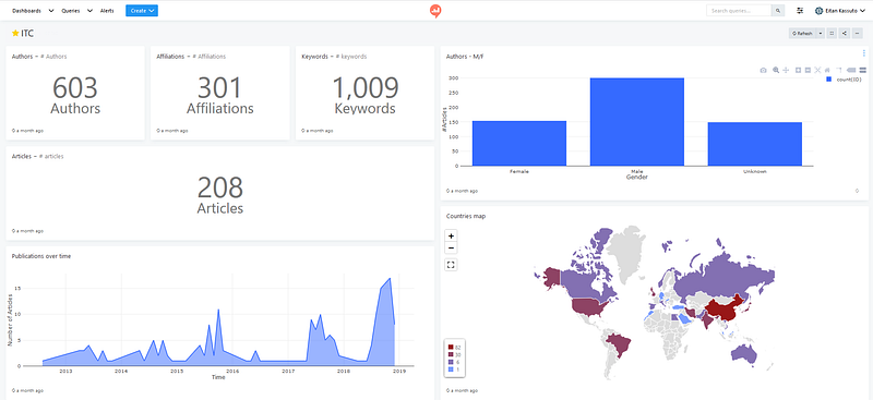
Before moving on, here is an overview of the data we collected for the topic “Neural Networks”.

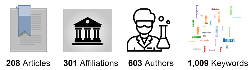
As you can see, not a lot of data was retrieved — this was because of the limited time we had available on the AWS (Amazon Web Services) machines. Due to the lack of sufficient data, the reader should evaluate the results with a pinch of salt — this is at this stage a proof of concept and is by no means a finished product.

Addressing the use cases above — High level trends:

For the high level trends we simply plotted the number of research papers published per month for the past 5 years.

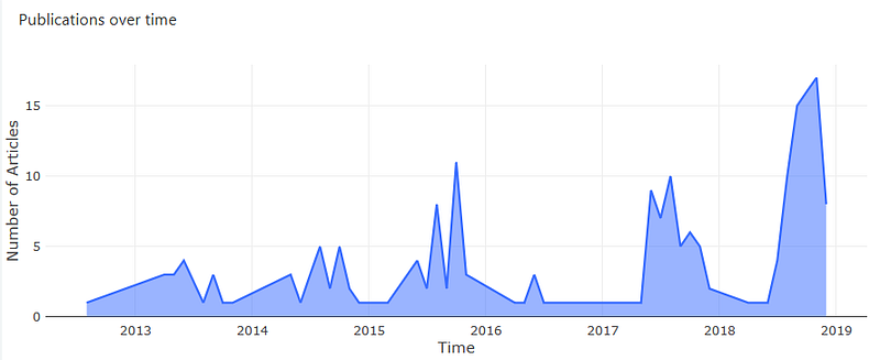
SELECT publication_date, count(id) AS num 
FROM articles 
GROUP BY publication_date 
ORDER BY publication_date;

Gender Distribution

This visualization makes use of enriched author data from genderize to view the gender distribution of authors within the specified topic. As seen in the figure below there are a large proportion of authors whose gender are unknown due to limitations of the genderize API.

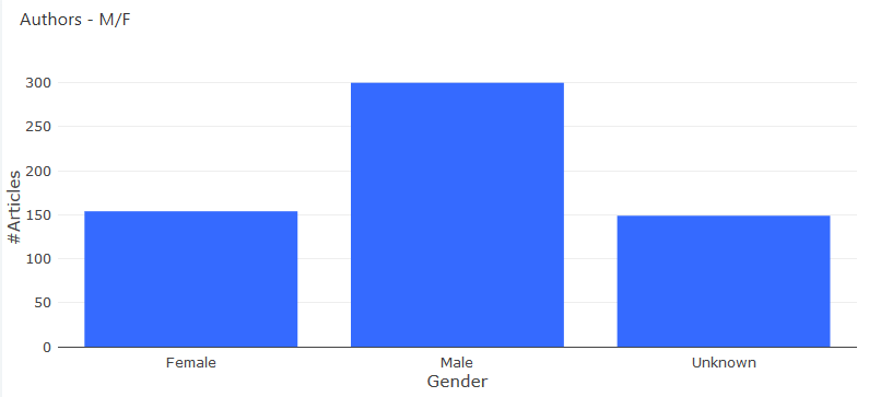
SELECT gender, count(ID) 
FROM authors 
GROUP BY gender;

Identifying leading countries in the field

When scraping affiliations for each author we were able to extract the country of each one, allowing us to create the visualization below. China publishes the majority of research papers for the topic “Neural Networks” as is expected due to their keen interest in AI. This information could be interesting for policy makers since one can track the advancements in AI in leading countries. Firstly, it can be helpful to monitor these leading countries to find opportunities for partnership in order to advance AI in both countries. Secondly, policy makers can use these insights in order to emulate leading countries in advancing AI within their own country.

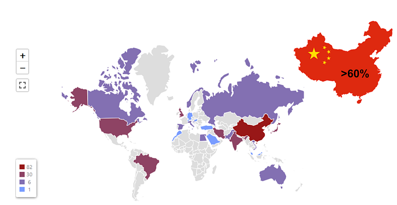
SELECT country, count(affiliation_id) AS counter
FROM affiliations 
GROUP BY country 
ORDER BY counter DESC;

Identifying top lead authors in the field

As a first approach to identifying the top researchers we decided to to compare the lead authors with the most citations associated to their name.

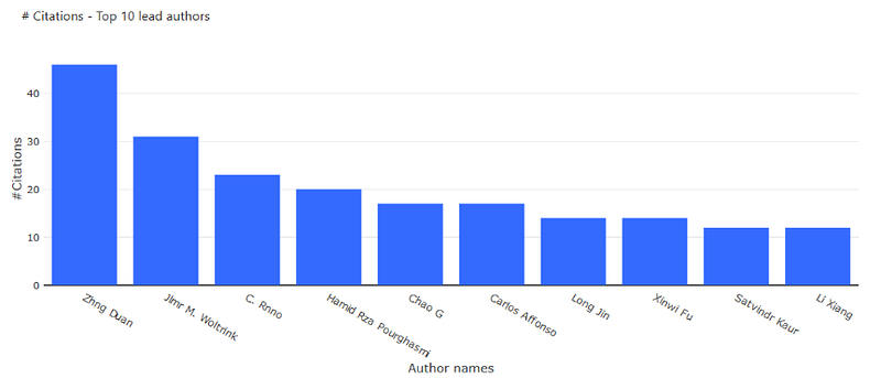
SELECT CONCAT(authors.first_name,” “, authors.last_name) AS name, SUM(articles.citations) AS num_citations 
FROM authors JOIN authors_article_junction JOIN articles
WHERE authors_article_junction.author_ID = authors.ID AND articles.ID = authors_article_junction.article_ID 
 AND authors_article_junction.importance = 1 
GROUP BY authors.ID 
ORDER BY num_citations DESC 
LIMIT 10;

Keywords map

The larger the word, the more frequent it is in the database

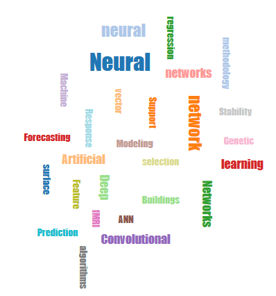
SELECT keywords.keyword_name, COUNT(keywords_ID) AS num 
FROM keyword_article_junction JOIN keywords 
WHERE keyword_article_junction.keywords_ID = keywords.ID 
GROUP BY keywords.keyword_name 
ORDER BY num DESC 
LIMIT 20;

Snapshot of our dashboard in Redash

Conclusion

We have reached the end of our Web Scraping with Python A — Z series. In our first post we gave a brief introduction of web scraping and spoke about more advanced techniques on how to avoid being blocked by a website. Also, we showed how one can use API calls in order to enrich the data to extract further insights. And lastly, in this post we showed how to create a database for storing the data obtained from web scraping and how to visualize this data using an open source tool — Redash.